Kirchhoff’s circuit laws are two equalities that deal with the current and potential difference (commonly known as voltage) in the lumped element model of electrical circuits. They were first described in 1845 byGustav Kirchhoff.[1] This generalized the work of Georg Ohm and preceded the work of Maxwell. Widely used in electrical engineering, they are also called Kirchhoff’s rules or simply Kirchhoff’s laws.
Both of Kirchhoff’s laws can be understood as corollaries of the Maxwell equations in the low-frequency limit. They are accurate for DC circuits, and for AC circuits at frequencies where the wavelengths of electromagnetic radiation are very large compared to the circuits.
Kirchhoff’s current law (KCL)

The current entering any junction is equal to the current leaving that junction. i2 + i3 = i1 + i4
This law is also called Kirchhoff’s first law, Kirchhoff’s point rule, or Kirchhoff’s junction rule (or nodal rule).
The principle of conservation of electric charge implies that:
- At any node (junction) in an electrical circuit, the sum of currents flowing into that node is equal to the sum of currents flowing out of that node, or:
- The algebraic sum of currents in a network of conductors meeting at a point is zero.
Recalling that current is a signed (positive or negative) quantity reflecting direction towards or away from a node, this principle can be stated as:

n is the total number of branches with currents flowing towards or away from the node.
This formula is valid for complex currents:

The law is based on the conservation of charge whereby the charge (measured in coulombs) is the product of the current (in amperes) and the time (in seconds).
Uses[edit]
A matrix version of Kirchhoff’s current law is the basis of most circuit simulation software, such as SPICE. Kirchhoff’s current law combined with Ohm’s Law is used in nodal analysis.
Kirchhoff’s voltage law (KVL)

The sum of all the voltages around the loop is equal to zero. v1+ v2 + v3 – v4 = 0
This law is also called Kirchhoff’s second law, Kirchhoff’s loop (or mesh) rule, and Kirchhoff’s second rule.
The principle of conservation of energy implies that
- The directed sum of the electrical potential differences (voltage) around any closed network is zero, or:
Similarly to KCL, it can be stated as:

Here, n is the total number of voltages measured. The voltages may also be complex:

This law is based on the conservation of energy whereby voltage is defined as the energy per unit charge. The total amount of energy gained per unit charge must equal the amount of energy lost per unit charge, as energy and charge are both conserved.
Generalization
In the low-frequency limit, the voltage drop around any loop is zero. This includes imaginary loops arranged arbitrarily in space – not limited to the loops delineated by the circuit elements and conductors. In the low-frequency limit, this is a corollary of Faraday’s law of induction (which is one of the Maxwell equations).
This has practical application in situations involving “static electricity“.
Limitations
KCL and KVL both depend on the lumped element model being applicable to the circuit in question. When the model is not applicable, the laws do not apply.
KCL, in its usual form, is dependent on the assumption that current flows only in conductors, and that whenever current flows into one end of a conductor it immediately flows out the other end. This is not a safe assumption for high-frequency AC circuits, where the lumped element model is no longer applicable.[2] It is often possible to improve the applicability of KCL by considering “parasitic capacitances” distributed along the conductors.[2] Significant violations of KCL can occur[3][4] even at 60Hz, which is not a very high frequency.
In other words, KCL is valid only if the total electric charge,  , remains constant in the region being considered. In practical cases this is always so when KCL is applied at a geometric point. When investigating a finite region, however, it is possible that the charge density within the region may change. Since charge is conserved, this can only come about by a flow of charge across the region boundary. This flow represents a net current, and KCL is violated.
KVL is based on the assumption that there is no fluctuating magnetic field linking the closed loop. This is not a safe assumption for high-frequency (short-wavelength) AC circuits.[2] In the presence of a changing magnetic field the electric field is not a conservative vector field. Therefore the electric field cannot be the gradient of any potential. That is to say, the line integral of the electric field around the loop is not zero, directly contradicting KVL.
It is often possible to improve the applicability of KVL by considering “parasitic inductances” (including mutual inductances) distributed along the conductors.[2] These are treated as imaginary circuit elements that produce a voltage drop equal to the rate-of-change of the flux.
Example

Assume an electric network consisting of two voltage sources and three resistors.
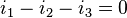
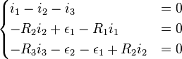
According to the first law we have
The second law applied to the closed circuit s1 gives

The second law applied to the closed circuit s2 gives

Thus we get a linear system of equations in  :
:
Assuming

the solution is

 has a negative sign, which means that the direction of is opposite to the assumed direction (the direction defined in the picture).