Lagrangian Mechanics - TheOldScientist

Lagrangian mechanics is a re-formulation of classical mechanics using the principle of stationary action (also called the principle of least action).^[1] Lagrangian mechanics applies to systems whether or not they conserve energy or momentum, and it provides conditions under which energy, momentum or both are conserved.^[2] It was introduced by the Italian-French mathematician Joseph-Louis Lagrange in 1788.

In Lagrangian mechanics, the trajectory of a system of particles is derived by solving the Lagrange equations in one of two forms, either the Lagrange equations of the first kind,^[3] which treat constraints explicitly as extra equations, often using Lagrange multipliers;^[4]^[5] or the Lagrange equations of the second kind, which incorporate the constraints directly by judicious choice of generalized coordinates.^[3]^[6] The fundamental lemma of the calculus of variations shows that solving the Lagrange equations is equivalent to finding the path for which the action functional is stationary, a quantity that is the integral of the Lagrangian over time.

The use of generalized coordinates may considerably simplify a system’s analysis. For example, consider a small frictionless bead traveling in a groove. If one is tracking the bead as a particle, calculation of the motion of the bead using Newtonian mechanics would require solving for the time-varying constraint force required to keep the bead in the groove. For the same problem using Lagrangian mechanics, one looks at the path of the groove and chooses a set of independent generalized coordinates that completely characterize the possible motion of the bead. This choice eliminates the need for the constraint force to enter into the resultant system of equations. There are fewer equations since one is not directly calculating the influence of the groove on the bead at a given moment.

Conceptual framework

Generalized coordinates

Illustration of a generalized coordinate q for one degree of freedom, of a particle moving in a complicated path. Four possibilities of q for the particle’s path are shown. For more particles each with their own degrees of freedom, there are more coordinates.

Concepts and terminology

For one particle acted on by external forces, Newton’s second law forms a set of 3 second-order ordinary differential equations, one for each dimension. Therefore, the motion of the particle can be completely described by 6 independent variables: 3 initial position coordinates and 3 initial velocity coordinates. Given these, the general solutions to Newton’s second law become particular solutions that determine the time evolution of the particle’s behaviour after its initial state (t = 0).

The most familiar set of variables for position r = (r₁, r₂, r₃) and velocity $\mathbf{\dot{r}}_j = (\dot{r}_1, \dot{r}_2, \dot{r}_3)$ are Cartesian coordinates and their time derivatives (i.e. position (x, y, z) and velocity (v_x, v_y, v_z) components). Determining forces in terms of standard coordinates can be complicated, and usually requires much labour.

An alternative and more efficient approach is to use only as many coordinates as are needed to define the position of the particle, at the same time incorporating the constraints on the system, and writing down kinetic and potential energies. In other words, to determine the number of degrees of freedomthe particle has, i.e. the number of possible ways the system can move subject to the constraints (forces that prevent it moving in certain paths). Energies are much easier to write down and calculate than forces, since energy is a scalar while forces are vectors.

These coordinates are generalized coordinates, denoted $q_j$ , and there is one for each degree of freedom. Their corresponding time derivatives are thegeneralized velocities, $\dot{q_j}$ . The number of degrees of freedom is usually not equal to the number of spatial dimensions: multi-body systems in 3-dimensional space (such as Barton’s Pendulums, planets in the solar system, or atoms in molecules) can have many more degrees of freedom incorporating rotations as well as translations. This contrasts the number of spatial coordinates used with Newton’s laws above.

Mathematical formulation

The position vector r in a standard coordinate system (like Cartesian, spherical etc.), is related to the generalized coordinates by some transformation equation:

\bold{r} = \bold{r}(q_i, t). \,

where there are as many q_i as needed (number of degrees of freedom in the system). Likewise for velocity and generalized velocities.

For example, for a simple pendulum of length ℓ, there is the constraint of the pendulum bob’s suspension (rod/wire/string etc.). The position r depends on the x and y coordinates at time t, that is, r(t)=(x(t),y(t)), however x and y are coupled to each other in a constraint equation (if x changes y must change, and vice versa). A logical choice for a generalized coordinate is the angle of the pendulum from vertical, θ, so we haver = (x(θ), y(θ)) = r(θ), in which θ = θ(t). Then the transformation equation would be

\bold{r}(\theta(t)) =(\ell\sin\theta, -\ell\cos\theta)

and so

\bold{\dot{r}}(\theta(t),\dot{\theta}(t))=( \ell\, \dot{\theta}\cos\theta, \ell\,\dot{\theta}\sin \theta)

which corresponds to the one degree of freedom the pendulum has. The term “generalized coordinates” is really a holdover from the period when Cartesian coordinates were the default coordinate system.

In general, from m independent generalized coordinates q_j, the following transformation equations hold for a system composed of n particles:^[7]^:260

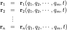
\begin{array}{r c l} \mathbf{r}_1 &=& \mathbf{r}_1(q_1, q_2, \cdots, q_m, t) \\ \mathbf{r}_2 &=& \mathbf{r}_2(q_1, q_2, \cdots, q_m, t) \\ & \vdots & \\ \mathbf{r}_n &=& \mathbf{r}_n(q_1, q_2, \cdots, q_m, t) \end{array}

where m indicates the total number of generalized coordinates. An expression for the virtual displacement (infinitesimal), δr_i of the system for time-independent constraints or “velocity-dependent constraints” is the same form as a total differential^[7]^:264

\delta \mathbf{r}_i = \sum_{j=1}^m \frac {\partial \mathbf {r}_i} {\partial q_j} \delta q_j,

where j is an integer label corresponding to a generalized coordinate.

The generalized coordinates form a discrete set of variables that define the configuration of a system. The continuum analogue for defining a field are field variables, say ϕ(r, t), which represents density function varying with position and time.

D’Alembert’s principle and generalized forces

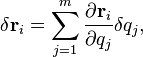
D’Alembert’s principle introduces the concept of virtual work due to applied forces F_i and inertial forces, acting on a three-dimensional accelerating system of n particles whose motion is consistent with its constraints,^[7]^:269

Mathematically the virtual work done δW on a particle of mass m_i through a virtual displacement δr_i (consistent with the constraints) is:

D’Alembert’s principle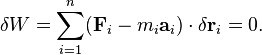

\delta W = \sum_{i=1}^n ( \mathbf {F}_{i} - m_i \mathbf{a}_i )\cdot \delta \mathbf r_i = 0.

where a_i are the accelerations of the particles in the system and i = 1, 2,…,n simply labels the particles. In terms of generalized coordinates

\delta W = \sum_{j=1}^m \sum_{i=1}^n ( \mathbf {F}_{i} - m_i \mathbf{a}_i )\cdot \frac {\partial \mathbf {r}_i} {\partial q_j} \delta q_j= 0.

this expression suggests that the applied forces may be expressed as generalized forces, Q_j. Dividing by δq_j gives the definition of a generalized force:^[7]^:265

Q_j = \frac{\delta W}{\delta q_j}= \sum_{i=1}^n \mathbf {F}_i \cdot \frac {\partial \mathbf{r}_i} {\partial q_j}.

If the forces F_i are conservative, there is a scalar potential field V in which the gradient of V is the force:^[7]^{:266 & 270}

\mathbf F_i = - \nabla V \Rightarrow Q_j = - \sum_{i=1}^n \nabla V \cdot \frac {\partial \mathbf {r}_i} {\partial q_j} = - \frac {\partial V}{\partial q_j}.

i.e. generalized forces can be reduced to a potential gradient in terms of generalized coordinates. The previous result may be easier to see by recognizing that V is a function of the r_i, which are in turn functions of q_j, and then applying the chain rule to the derivative of $V$ with respect to q_j.

Kinetic energy relations

The kinetic energy, T, for the system of particles is defined by^[7]^:269

T = \frac {1}{2} \sum_{i=1}^n m_i \mathbf {\dot{r}}_i \cdot \mathbf {\dot{r}}_i.

The partial derivatives of T with respect to the generalized coordinates q_j and generalized velocities $\dot{q}_j$ are ^[7]^:269:

\frac{\partial T}{\partial q_j} = \sum_{i=1}^n m_i \mathbf{\dot{r}}_i \cdot \frac{\partial \mathbf{\dot{r}}_i}{\partial q_j}

\quad \frac{\partial T}{\partial \dot{q}_j} = \sum_{i=1}^n m_i \mathbf{\dot{r}}_i \cdot \frac{\partial \mathbf{\dot{r}}_i}{\partial \dot{q}_j}.

Because $\dot{q_j}$ and $q_j$ are independent variables:

\frac {\partial \mathbf{\dot{r}}_i}{\partial \dot{q_j}} = \frac {\partial \mathbf{r}_i}{\partial q_j} .

Then:

\quad \frac{\partial T}{\partial \dot{q}_j} = \sum_{i=1}^n m_i \mathbf{\dot{r}}_i \cdot \frac{\partial \mathbf{r}_i}{\partial q_j} \ .

The total time derivative of this equation is

\frac{\mathrm{d}}{\mathrm{d}t}\frac{\partial T}{\partial \dot{q}_j} = \sum_{i=1}^n m_i \mathbf{\ddot{r}}_i \cdot \frac {\partial \mathbf{r}_i}{\partial q_j} + \sum_{i=1}^n m_i \mathbf{\dot{r}}_i \cdot \frac {\partial \mathbf{\dot{r}}_i}{\partial q_j} = Q_j + \frac{\partial T}{\partial q_j} \ .

resulting in:

Generalized equations of motion

Q_j = \frac{\mathrm{d}}{\mathrm{d}t} \left ( \frac {\partial T}{\partial \dot{q}_j} \right ) - \frac {\partial T}{\partial q_j}

Newton’s laws are contained in it, yet there is no need to find the constraint forces because virtual work and generalized coordinates (which account for constraints) are used. This equation in itself is not actually used in practice, but is a step towards deriving Lagrange’s equations (see below).^[8]

Lagrangian and action

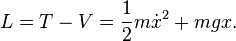
The core element of Lagrangian mechanics is the Lagrangian function, which summarizes the dynamics of the entire system in a very simple expression. The physics of analyzing a system is reduced to choosing the most convenient set of generalized coordinates, determining the kinetic and potential energies of the constituents of the system, then writing down the equation for the Lagrangian to use in Lagrange’s equations. It is defined by ^[9]

L = T - V \,

where T is the total kinetic energy and V is the total potential energy of the system.

The next fundamental element is the action $\mathcal{S}$ , defined as the time integral of the Lagrangian:^[8]

\mathcal{S} = \int_{t_1}^{t_2} L\,\mathrm{d}t.

This also contains the dynamics of the system, and has deep theoretical implications (discussed below). Technically action is a functional, rather than a function: its value depends on the full Lagrangian function for all times between t₁ and t₂. Its dimensions are the same as angular momentum.

In classical field theory, the physical system is not a set of discrete particles, but rather a continuous field defined over a region of 3d space. Associated with the field is a Lagrangian density $\mathcal{L}(\mathbf{r},t)$ defined in terms of the field and its derivatives at a location $\mathbf{r}$ . The total Lagrangian is then the integral of the Lagrangian density over 3d space (see volume integral):

L(t) = \int \mathcal{L}(\mathbf{r},t) \mathrm{d}^3 \mathbf{r} \,

where d³r is a 3d differential volume element, must be used instead. The action becomes an integral over space and time:

\mathcal{S} = \int_{t_1}^{t_2}\int \mathcal{L}(\mathbf{r},t) \mathrm{d}^3\mathbf{r} \mathrm{d}t.

Hamilton’s principle of stationary action

Let q₀ and q₁ be the coordinates at respective initial and final times t₀ and t₁. Using the calculus of variations, it can be shown that Lagrange’s equations are equivalent to Hamilton’s principle:

The trajectory of the system between t₀ and t₁ has a stationary action S.

By stationary, we mean that the action does not vary to first-order from infinitesimal deformations of the trajectory, with the end-points (q₀, t₀) and (q₁,t₁) fixed. Hamilton’s principle can be written as:

\delta \mathcal{S} = 0. \,\!

Thus, instead of thinking about particles accelerating in response to applied forces, one might think of them picking out the path with a stationary action.

Hamilton’s principle is sometimes referred to as the principle of least action, however the action functional need only be stationary, not necessarily a maximum or a minimum value. Any variation of the functional gives an increase in the functional integral of the action.

We can use this principle instead of Newton’s Laws as the fundamental principle of mechanics, this allows us to use an integral principle (Newton’s Laws are based on differential equations so they are a differential principle) as the basis for mechanics. However it is not widely stated that Hamilton’s principle is a variational principle only with holonomic constraints, if we are dealing with nonholonomic systems then the variational principle should be replaced with one involving d’Alembert principle of virtual work. Working only with holonomic constraints is the price we have to pay for using an elegant variational formulation of mechanics.

Lagrange equations of the first kind

Lagrange introduced an analytical method for finding stationary points using the method of Lagrange multipliers, and also applied it to mechanics.

For a system subject to the constraint equation on the generalized coordinates:

F(r_1,r_2,r_3) = A

where A is a constant, then Lagrange’s equations of the first kind are:

\left[\frac{\partial L}{\partial r_j} - \frac{\mathrm{d}}{\mathrm{d}t}\left(\frac{\partial L}{\partial \dot{r}_j}\right)\right] + \lambda\frac{\partial F}{\partial r_j}=0

where λ is the Lagrange multiplier. By analogy with the mathematical procedure, we can write:

\frac{\delta L}{\delta r_j} + \lambda\frac{\partial F}{\partial r_j}=0

where

\frac{\delta L}{\delta r_j} = \frac{\partial L}{\partial r_j} - \frac{\mathrm{d}}{\mathrm{d}t}\left(\frac{\partial L}{\partial \dot{r}_j}\right)

denotes the variational derivative.

For e constraint equations F₁, F₂,…, F_e, there is a Lagrange multiplier for each constraint equation, and Lagrange’s equations of the first kind generalize to:

Lagrange’s equations (1st kind)

\frac{\delta L}{\delta r_j} + \sum_{i=1}^e \lambda_i\frac{\partial F_i}{\partial r_j}=0

This procedure does increase the number of equations, but there are enough to solve for all of the multipliers. The number of equations generated is the number of constraint equations plus the number of coordinates, i.e. e + m. The advantage of the method is that (potentially complicated) substitution and elimination of variables linked by constraint equations can be bypassed.

There is a connection between the constraint equations F_j and the constraint forces N_j acting in the conservative system (forces are conservative):

N_j = \sum_{i=1}^e \lambda_i \frac{\partial F_i}{\partial r_j}

which is derived below.

[show]Derivation of connection between constraint equations and forces

Lagrange equations of the second kind

Euler–Lagrange equations

For any system with m degrees of freedom, the Lagrange equations include m generalized coordinates and m generalized velocities. Below, we sketch out the derivation of the Lagrange equations of the second kind. In this context, V is used rather than U for potential energy and T replaces K for kinetic energy. See the references for more detailed and more general derivations.

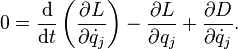
The equations of motion in Lagrangian mechanics are the Lagrange equations of the second kind, also known as the Euler–Lagrange equations:^[8]^[10]

Lagrange’s equations (2nd kind)

\frac{\mathrm{d}}{\mathrm{d}t} \left ( \frac {\partial L}{\partial \dot{q}_j} \right ) = \frac {\partial L}{\partial q_j}

where j = 1, 2,…m represents the jth degree of freedom, q_j are the generalized coordinates, and $\dot{q}_j$ are the generalized velocities.

Although the mathematics required for Lagrange’s equations appears significantly more complicated than Newton’s laws, this does point to deeper insights into classical mechanics than Newton’s laws alone: in particular, symmetry and conservation. In practice it’s often easier to solve a problem using the Lagrange equations than Newton’s laws, because the minimum generalized coordinates q_i can be chosen by convenience to exploit symmetries in the system, and constraint forces are incorporated into the geometry of the problem. There is one Lagrange equation for each generalized coordinate q_i.

For a system of many particles, each particle can have different numbers of degrees of freedom from the others. In each of the Lagrange equations, T is the total kinetic energy of the system, and V the total potential energy.

Derivation of Lagrange’s equations

Hamilton’s principle

The Euler–Lagrange equations follow directly from Hamilton’s principle, and are mathematically equivalent. From the calculus of variations, any functional of the form:

J=\int_{x_1}^{x_2}F(x,y,y')\mathrm{d}x

leads to the general Euler–Lagrange equation for stationary value of J. (see main article for derivation):

\frac{\mathrm{d}}{\mathrm{d}x}\frac{\partial F}{\partial y'}=\frac{\partial F}{\partial y}

Then making the replacements:

x\rightarrow t,\quad y\rightarrow q,\quad y'\rightarrow \dot{q},\quad F\rightarrow L,\quad J\rightarrow\mathcal{S}

yields the Lagrange equations for mechanics. Since mathematically Hamilton’s equations can be derived from Lagrange’s equations (by a Legendre transformation) and Lagrange’s equations can be derived from Newton’s laws, all of which are equivalent and summarize classical mechanics, this means classical mechanics is fundamentally ruled by a variation principle (Hamilton’s principle above).

Generalized forces

For a conservative system, since the potential field is only a function of position, not velocity, Lagrange’s equations also follow directly from the equation of motion above:

Q_j = \frac{\mathrm{d}}{\mathrm{d}t} \left ( \frac {\partial \mathcal (L+V)}{\partial \dot{q}_j} \right ) - \frac {\partial \mathcal (L+V)}{\partial q_j} = \left[\frac{\mathrm{d}}{\mathrm{d}t}\left ( \frac {\partial L}{\partial \dot{q}_j} \right ) +0\right] - \left[ \frac {\partial L}{\partial q_j}+\frac {\partial V}{\partial q_j}\right] = \frac{\mathrm{d}}{\mathrm{d}t}\left ( \frac {\partial L}{\partial \dot{q}_j} \right ) - \frac {\partial L}{\partial q_j} + Q_j.

simplifying to

\frac{\mathrm{d}}{\mathrm{d}t}\left ( \frac {\partial L}{\partial \dot{q}_j} \right ) = \frac {\partial L}{\partial q_j}

This is consistent with the results derived above and may be seen by differentiating the right side of the Lagrangian with respect to $\dot{q}_j$ and time, and solely with respect to q_j, adding the results and associating terms with the equations for F_i and Q_j.

Newton’s laws[edit]

As the following derivation shows, no new physics is introduced, so the Lagrange equations can describe the dynamics of a classical system equivalently as Newton’s laws.

[show]Derivation of Lagrange’s equations from Newton’s 2nd law and D’Alembert’s principle

When q_i = r_i (i.e. the generalized coordinates are simply the Cartesian coordinates), it is straightforward to check that Lagrange’s equations reduce to Newton’s second law.

Dissipation function

Main article: Rayleigh dissipation function

In a more general formulation, the forces could be both potential and viscous. If an appropriate transformation can be found from the F_i, Rayleigh suggests using a dissipation function, D, of the following form:^[7]^:271

D = \frac {1}{2} \sum_{j=1}^m \sum_{k=1}^m C_{j k} \dot{q}_j \dot{q}_k.

where C_jk are constants that are related to the damping coefficients in the physical system, though not necessarily equal to them

If D is defined this way, then^[7]^:271

Q_j = - \frac {\partial V}{\partial q_j} - \frac {\partial D}{\partial \dot{q}_j}

and

0 = \frac{\mathrm{d}}{\mathrm{d}t} \left ( \frac {\partial L}{\partial \dot{q}_j} \right ) - \frac {\partial L}{\partial q_j} + \frac {\partial D}{\partial \dot{q}_j}.

Examples

In this section two examples are provided in which the above concepts are applied. The first example establishes that in a simple case, the Newtonian approach and the Lagrangian formalism agree. The second case illustrates the power of the above formalism, in a case that is hard to solve with Newton’s laws.

Falling mass

Consider a point mass m falling freely from rest. By gravity a force F = mg is exerted on the mass (assuming g constant during the motion). Filling in the force in Newton’s law, we find $\ddot x = g$ from which the solution

x(t) = \frac{1}{2} g t^2

follows (by taking the antiderivative of the antiderivative, and choosing the origin as the starting point). This result can also be derived through the Lagrangian formalism. Take x to be the coordinate, which is 0 at the starting point. The kinetic energy is T = ¹⁄₂mv² and the potential energy is V = −mgx; hence,

L = T - V = \frac{1}{2} m \dot{x}^2 + m g x.

Then

0 = \frac{\partial L}{\partial x} - \frac{\mathrm{d}}{\mathrm{d}t} \frac{\partial L}{\partial \dot x} = m g - m \frac{\mathrm{d} \dot x}{\mathrm{d} t}

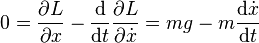
which can be rewritten as $\ddot x = g$ , yielding the same result as earlier.

Pendulum on a movable support

Consider a pendulum of mass m and length ℓ, which is attached to a support with mass M, which can move along a line in the x-direction. Let x be the coordinate along the line of the support, and let us denote the position of the pendulum by the angle θ from the vertical.

Sketch of the situation with definition of the coordinates (click to enlarge)

The kinetic energy can then be shown to be

\begin{array}{rcl} T &=& \frac{1}{2} M \dot{x}^2 + \frac{1}{2} m \left( \dot{x}_\mathrm{pend}^2 + \dot{y}_\mathrm{pend}^2 \right) \\ &=& \frac{1}{2} M \dot{x}^2 + \frac{1}{2} m \left[ \left( \dot x + \ell \dot\theta \cos \theta \right)^2 + \left( \ell \dot\theta \sin \theta \right)^2 \right], \end{array}

and the potential energy of the system is

V = m g y_\mathrm{pend} = - m g \ell \cos \theta .

The Lagrangian is therefore

\begin{array}{rcl} L &=& T - V \\ &=& \frac{1}{2} M \dot{x}^2 + \frac{1}{2} m \left[ \left( \dot x + \ell \dot\theta \cos \theta \right)^2 + \left( \ell \dot\theta \sin \theta \right)^2 \right] + m g \ell \cos \theta \\ &=& \frac{1}{2} \left( M + m \right) \dot x^2 + m \dot x \ell \dot \theta \cos \theta + \frac{1}{2} m \ell^2 \dot \theta ^2 + m g \ell \cos \theta \end{array}

Now carrying out the differentiations gives for the support coordinate x

\frac{\mathrm{d}}{\mathrm{d}t} \left[ (M + m) \dot x + m \ell \dot\theta \cos\theta \right] = 0,

therefore:

(M + m) \ddot x + m \ell \ddot\theta\cos\theta-m \ell \dot\theta ^2 \sin\theta = 0

indicating the presence of a constant of motion. Performing the same procedure for the variable $\theta$ yields:

\frac{\mathrm{d}}{\mathrm{d}t}\left[ m( \dot x \ell \cos\theta + \ell^2 \dot\theta ) \right] + m \ell (\dot x \dot \theta + g) \sin\theta = 0;

therefore

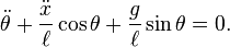
\ddot\theta + \frac{\ddot x}{\ell} \cos\theta + \frac{g}{\ell} \sin\theta = 0.\,

These equations may look quite complicated, but finding them with Newton’s laws would have required carefully identifying all forces, which would have been much more laborious and prone to errors. By considering limit cases, the correctness of this system can be verified: For example, $\ddot x \to 0$ should give the equations of motion for a pendulum that is at rest in some inertial frame, while $\ddot\theta \to 0$ should give the equations for a pendulum in a constantly accelerating system, etc. Furthermore, it is trivial to obtain the results numerically, given suitable starting conditions and a chosen time step, by stepping through the results iteratively.

Two-body central force problem

The basic problem is that of two bodies in orbit about each other attracted by a central force. The Jacobi coordinates are introduced; namely, the location of the center of mass R and the separation of the bodies r(the relative position). The Lagrangian is then^[11]^[12]

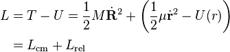
\begin{align} L &= T-U = \frac {1}{2} M \dot{\mathbf{R}}^2 + \left( \frac {1}{2} \mu \dot{\mathbf{r}}^2 - U(r) \right) \\ &= L_{\mathrm{cm}} + L_{\mathrm{rel}} \end{align}

where M is the total mass, μ is the reduced mass, and U the potential of the radial force. The Lagrangian is divided into a center-of-mass term and a relative motion term. The R equation from the Euler–Lagrange system is simply:

M\ddot{\mathbf{R}} = 0, \,

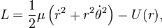
resulting in simple motion of the center of mass in a straight line at constant velocity. The relative motion is expressed in polar coordinates (r, θ):

L=\frac{1}{2} \mu \left(\dot r ^2 +r^2 \dot \theta ^2 \right) - U(r),

which does not depend upon θ, therefore an ignorable coordinate. The Lagrange equation for θ is then:

\frac {\partial L}{\partial \dot \theta} = \mu r^2 \dot \theta = \mathrm{constant} = \ell, \,

where ℓ is the conserved angular momentum. The Lagrange equation for r is:

\frac{\partial L}{\partial r} = \frac{\mathrm{d}}{\mathrm{d}t} \frac{\partial L}{\partial \dot r}, \,

or:

\mu r \dot \theta ^2 -\frac {dU}{dr} = \mu \ddot r. \,

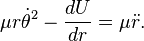
This equation is identical to the radial equation obtained using Newton’s laws in a co-rotating reference frame, that is, a frame rotating with the reduced mass so it appears stationary. If the angular velocity is replaced by its value in terms of the angular momentum,

\dot \theta = \frac {\ell}{\mu r^2}, \,

the radial equation becomes:^[13]

\mu \ddot r = -\frac{dU}{dr} + \frac{\ell^2}{\mu r^3}. \,

which is the equation of motion for a one-dimensional problem in which a particle of mass μ is subjected to the inward central force −dU/dr and a second outward force, called in this context the centrifugal force:

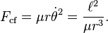
F_{\mathrm{cf}} = \mu r \dot \theta ^2 = \frac {\ell^2}{\mu r^3}. \,

Of course, if one remains entirely within the one-dimensional formulation, ℓ enters only as some imposed parameter of the external outward force, and its interpretation as angular momentum depends upon the more general two-dimensional problem from which the one-dimensional problem originated.

If one arrives at this equation using Newtonian mechanics in a co-rotating frame, the interpretation is evident as the centrifugal force in that frame due to the rotation of the frame itself. If one arrives at this equation directly by using the generalized coordinates (r, θ) and simply following the Lagrangian formulation without thinking about frames at all, the interpretation is that the centrifugal force is an outgrowth of using polar coordinates. As Hildebrand says:^[14] “Since such quantities are not true physical forces, they are often called inertia forces. Their presence or absence depends, not upon the particular problem at hand, but upon the coordinate system chosen.” In particular, if Cartesian coordinates are chosen, the centrifugal force disappears, and the formulation involves only the central force itself, which provides the centripetal force for a curved motion.

This viewpoint, that fictitious forces originate in the choice of coordinates, often is expressed by users of the Lagrangian method. This view arises naturally in the Lagrangian approach, because the frame of reference is (possibly unconsciously) selected by the choice of coordinates.^[15] Unfortunately, this usage of “inertial force” conflicts with the Newtonian idea of an inertial force. In the Newtonian view, an inertial force originates in the acceleration of the frame of observation (the fact that it is not an inertial frame of reference), not in the choice of coordinate system. To keep matters clear, it is safest to refer to the Lagrangian inertial forces asgeneralized inertial forces, to distinguish them from the Newtonian vector inertial forces. That is, one should avoid following Hildebrand when he says (p. 155) “we deal always with generalized forces, velocities accelerations, and momenta. For brevity, the adjective “generalized” will be omitted frequently.”

It is known that the Lagrangian of a system is not unique. Within the Lagrangian formalism the Newtonian fictitious forces can be identified by the existence of alternative Lagrangians in which the fictitious forces disappear, sometimes found by exploiting the symmetry of the system.^[16]

Extensions of Lagrangian mechanics

The Hamiltonian, denoted by H, is obtained by performing a Legendre transformation on the Lagrangian, which introduces new variables, canonically conjugate to the original variables. This doubles the number of variables, but makes differential equations first order. The Hamiltonian is the basis for an alternative formulation of classical mechanics known as Hamiltonian mechanics. It is a particularly ubiquitous quantity inquantum mechanics (see Hamiltonian (quantum mechanics)).

In 1948, Feynman discovered the path integral formulation extending the principle of least action to quantum mechanics for electrons and photons. In this formulation, particles travel every possible path between the initial and final states; the probability of a specific final state is obtained by summing over all possible trajectories leading to it. In the classical regime, the path integral formulation cleanly reproduces Hamilton’s principle, and Fermat’s principle in optics.

Dissipation (i.e. non-conservative systems) can also be treated with an effective Lagrangians formulated by a certain doubling of the degrees of freedom; see